- Packages I will use to read and plot the data
- Read the data in from part 1, part one did not function as wanted, so re-select desired countries and rename the 4th column to Marriage_rate.
Interactive graph
-Start with the data -group it by the Entity, or country -mutate Marriage_rate to only show 2 digits -have year start from the beggining of the year, not at the end as default -assign Year to the X axis -create the river effect with our data, set legend to false -Set title to Annual marriage rate by world entity -Set subtext to per 1,000 people -Set sublink to https://ourworldindata.org/marriages-and-divorces -Set theme to roma
regional_marriage %>%
  group_by(Entity)%>%
  mutate(Marriage_rate = round(Marriage_rate, 2),
         Year = paste(Year, "12", "31", sep = "-")) %>%
    e_charts(x=Year) %>%
    e_river(serie = Marriage_rate, legend= FALSE) %>%
    e_tooltip(trigger = "axis") %>%
    e_title(text = "Annual Marriage Rate, by World Entity",
            subtext = "(Per thousand people). Source: Our World in Data",
            sublink = "https://ourworldindata.org/marriages-and-divorces",
            left = "center") %>%
    e_theme("roma")
Static Graph
-Start with the data -use ggplot to create a new ggplot object -set the X axis of this object to year, the Yto marriage rate, and fill equivalent to entity -geom_area will display the marriage rate -scale_fill_discrete_divergingx is in the colorspace package, and it sets the colors to the roma theme, as well as selects a maximum of 4 colors for the regions -theme_classic sets the theme -theme(legend.position = “bottom”) puts the legend at the bottom of the plot -labs sets the y axis lable, fill = NULL indicates the fill var will not have the labelled Entity
regional_marriage %>%
  ggplot(aes(x = Year, y = Marriage_rate, fill = Entity))+
  geom_area()+
  colorspace::scale_fill_discrete_divergingx(palette = "roma", nmax = 4)+
  theme_classic()+
  theme(legend.position = "bottom")+
  labs(y = "in billions of tonnes", fill = NULL)
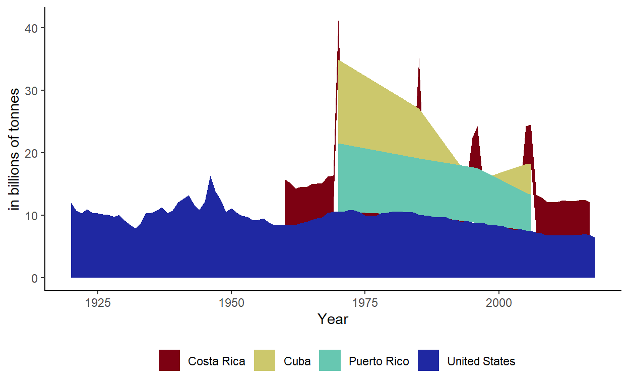
These plots show a decline in marriage rates since each country began tracking them.