Load the R packages
Download \(CO_2\) emissions per capita from Our world in Data into directory.
Assign the location of the file to file_csv. The data should be in the same directory as this file
read the data into R and assign it to emmisions
Show the First 10 rows (observations of) emissions
emissions
# A tibble: 23,307 x 4
   Entity      Code   Year `Annual CO2 emissions (per capita)`
   <chr>       <chr> <dbl>                               <dbl>
 1 Afghanistan AFG    1949                              0.0019
 2 Afghanistan AFG    1950                              0.0109
 3 Afghanistan AFG    1951                              0.0117
 4 Afghanistan AFG    1952                              0.0115
 5 Afghanistan AFG    1953                              0.0132
 6 Afghanistan AFG    1954                              0.013
 7 Afghanistan AFG    1955                              0.0186
 8 Afghanistan AFG    1956                              0.0218
 9 Afghanistan AFG    1957                              0.0343
10 Afghanistan AFG    1958                              0.038
# ... with 23,297 more rows
Start with emissions data THEN
-use clean_names from the janitor package -assign the output to tidy_emissions -show the first 10 rows of tidy_emissions
tidy_emissions <- emissions %>%
  clean_names()

tidy_emissions
# A tibble: 23,307 x 4
   entity      code   year annual_co2_emissions_per_capita
   <chr>       <chr> <dbl>                           <dbl>
 1 Afghanistan AFG    1949                          0.0019
 2 Afghanistan AFG    1950                          0.0109
 3 Afghanistan AFG    1951                          0.0117
 4 Afghanistan AFG    1952                          0.0115
 5 Afghanistan AFG    1953                          0.0132
 6 Afghanistan AFG    1954                          0.013
 7 Afghanistan AFG    1955                          0.0186
 8 Afghanistan AFG    1956                          0.0218
 9 Afghanistan AFG    1957                          0.0343
10 Afghanistan AFG    1958                          0.038
# ... with 23,297 more rows
Start with the tidy_emissions THEN -use filter to extracr rows with year == 2018 THEN -use skim to calculate the descriptive statistics
| Name | Piped data |
| Number of rows | 229 |
| Number of columns | 4 |
| _______________________ | |
| Column type frequency: | |
| character | 2 |
| numeric | 2 |
| ________________________ | |
| Group variables | None |
Variable type: character
| skim_variable | n_missing | complete_rate | min | max | empty | n_unique | whitespace |
|---|---|---|---|---|---|---|---|
| entity | 0 | 1.00 | 4 | 32 | 0 | 229 | 0 |
| code | 12 | 0.95 | 3 | 8 | 0 | 217 | 0 |
Variable type: numeric
| skim_variable | n_missing | complete_rate | mean | sd | p0 | p25 | p50 | p75 | p100 | hist |
|---|---|---|---|---|---|---|---|---|---|---|
| year | 0 | 1 | 2018.00 | 0.00 | 2018.00 | 2018.00 | 2018.0 | 2018.00 | 2018.00 | ▁▁▇▁▁ |
| annual_co2_emissions_per_capita | 0 | 1 | 5.03 | 5.63 | 0.03 | 0.99 | 3.5 | 6.85 | 38.44 | ▇▂▁▁▁ |
12observations have a missing code, how are these different? -start with tidy_emissions then extract rows with year == 2018 and are missing a code
# A tibble: 12 x 4
   entity                     code   year annual_co2_emissions_per_ca~
   <chr>                      <chr> <dbl>                        <dbl>
 1 Africa                     <NA>   2018                         1.09
 2 Asia                       <NA>   2018                         4.44
 3 Asia (excl. China & India) <NA>   2018                         4.14
 4 EU-27                      <NA>   2018                         6.85
 5 EU-28                      <NA>   2018                         6.70
 6 Europe                     <NA>   2018                         7.48
 7 Europe (excl. EU-27)       <NA>   2018                         8.39
 8 Europe (excl. EU-28)       <NA>   2018                         9.15
 9 North America              <NA>   2018                        11.4
10 North America (excl. USA)  <NA>   2018                         4.80
11 Oceania                    <NA>   2018                        11.4
12 South America              <NA>   2018                         2.58
Start with tidy_emissions THEN -use filter to extract rows with year == 2019 and without missing codes THEN -useselect to drop the year variable -use rename to change the variable entity to country -assign the output to emissions_2019
Which 15 countries have the highestper_capita_co2_emissions? -Start with emissions_2019 THEN -use slice_max to extract the 15 rows with the per_capita_co2_emissions -assign output to max_15_emitters
Which 15 countries have the lowest per_capita_co2_emissions? -start with emissions_2019 THEN -use slice_min to extract the 15 rows with lowest values -assign the output to min_15_emitters
Use bind_rows to bind together the max_15_emitters and min_15_emitters -assign the output to max_min_15
max_min_15 <- bind_rows(max_15_emitters,min_15_emitters)
Read the 3 file formats into R
max_min_15_csv <- read_csv("max_min_15.csv")
max_min_15_tsv <- read_tsv("max_min_15.tsv")
max_min_15_psv <- read_delim("max_min_15.psv", delim = "|")
Use setdiff to check for differences in max_min_, max_min_15_csv, and max_min_15_psv
setdiff(max_min_15_csv, max_min_15_tsv)
# A tibble: 0 x 3
# ... with 3 variables: country <chr>, code <chr>,
#   annual_co2_emissions_per_capita <dbl>
Any differences?
- Reorder country in max_min_15 for plotting and to assign to max_min_15_plot_data -start with emissions_2018 THEN -use mutate to reorder country according to per_capital_co2_emissions
16 Plot max_min_15_plot_data
17 save the plot directory with this postggplot(data = max_min_15_plot_data, mapping =aes(annual_co2_emissions_per_capita, country))+ geom_col()+ labs(title = "The top 15 and bottom 15 per capita c02 emissions", subtitle = "for 2018", x = NULL, y = NULL)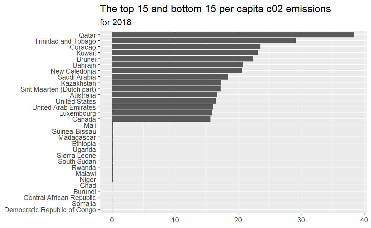
18 Add preview.png to yaml chuck at the top of this file
preview: preview.png